Advanced Building Features

In this section, we look at the special purpose building features designed for specific tasks and circumstances.

Using a Custom Fragment Library

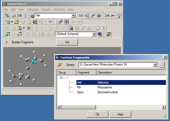
The Custom Fragment button can be used to access and modify a local fragment library. Clicking on it when it is inactive activates the last used custom fragment library; the first fragment within it becomes the current fragment, appearing in the area below the toolbars and in the popup menu to the right of the various building buttons. Clicking on the same button when it is selected opens the Custom Fragments palette, bringing up the window in Figure 28.

Figure 28. The Custom Fragments Window

This palette allows you to select from the available fragments in the open library. The selected fragment will become the current fragment once the dialog is exited.

The Library field at the top of the palette indicates the fragment library that is in use. Previously opened libraries are also present in the list. Additional library locations may be opened by clicking on the button labeled “...”.

Fragment libraries are simply folders on disk, and individual fragments within a library are stored as files within that folder. Thus, creating a new fragment library consists of creating a folder at the desired location and then selecting it in this palette. The library will obviously be initially empty. Any non-fragment files within the folder are ignored, although best practice is to limit fragment library folder use solely to fragment files.

Fragments within a fragment library are organized into a series of user-defined groups. If this feature has not been used, then all fragments will be within the “root” group: i.e., / as in the figure.

A context menu, reached by right clicking within the white fragment list area in the center of the palette, is used to manage and modify fragment libraries. It has the following selections:

• New Group: Create a new group within the current library. The group is initially given a generic name which you can modify. Control-G is equivalent to this menu selection (Command-N under Mac OS X).
• New Fragment From Active Molecule: Add the current molecule within the currently selected group within the current fragment library. A generic label and description will be set which you should edit as appropriate. In this context, Control-N/Command-N has the same function as this menu item.
• Edit Cell: Edit the text within the current item (group name, fragment name, fragment description). Note that the top level group name cannot be modified.
• Delete: Delete the currently selected fragment or fragment group. Note that the top-level fragment group cannot be deleted. The Delete key is equivalent to this menu item.

Note that fragments within a library can be updated only by removing and then readding them (there is no way to modify an existing fragment).

The Atom List Editor

The Atom List Editor window is displayed when you select the Edit=>Atom List menu item or click on the Atom List button. This tool presents the coordinates and other parameters for the molecule in the active View window in an editable spreadsheet format. The window’s default configuration is illustrated in Figure 29.

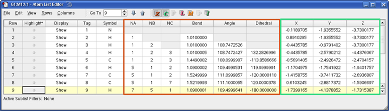
Figure 29. The Atom List Editor

The columns that are present in the table are controlled by the buttons in the toolbar. Columns corresponding to highlighted buttons are visible. Only buttons relevant to the current molecular structure are active. Individual columns may be displayed/hidden using the items on the Columns menu. You can also go directly to a specific atom (by number) using the Go To control in the toolbar.

The default configuration of this window displays the molecule’s Z-matrix and Cartesian coordinates. Different data can be selected for display using the toolbar buttons. From the left, they control Z-matrix coordinates (Z), Cartesian coordinates (C), fractional coordinates for PBC jobs (F), ONIOM layer assignments and related settings (L), Molecular Mechanics atoms types and other data (M), Isotope specification (I), and PDB file residue and chain data (P). Columns corresponding to the final button are read-only. Figure 26 illustrates the columns that may be present in this window. Clicking one of the lettered display icons will show or hide all columns in that group. You can also control the display of every individual column by selecting or deselecting it in the Columns menu.

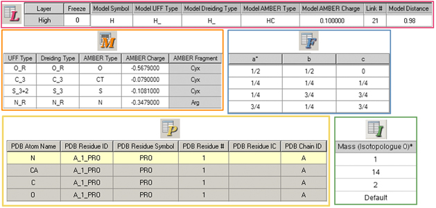
Figure 30. Additional Atom List Editor Columns

Beginning at the top and moving down and from left to right, these columns are controlled by the ONIOM Layers button, the Molecular Mechanics Parameters button, the Fractional Coordinates button, the PDB Info button, and the Isotope Masses button. Note that shaded columns are read-only.

Any of the molecular parameters can be edited in this spreadsheet-like window. Atoms may be selected by clicking on their Row cell in the leftmost column (and deselected by clicking it a second time). The dot in the Highlight column causes the corresponding atoms to also be selected/deselected in the molecule’s View window.

You can add additional atoms by scrolling to the bottom of the window, selecting an element in the Symbol column, and then clicking the Add button. This inserts a new row into the list (filled with default values, as in Figure 30 above).

The various menu items in the Atom List Editor window are described below. The File menu includes items related to saving and printing the data in the table:

• Export Data: Save the data as a tab-separated format text file.
• Print: Print the atom list table.
• Close: Close the Atom List Editor dialog.

The Edit menu items allow you to modify the contents of the molecule specification:

• Undo: Undo the previous action.
• Redo: Restore the previous “undone” operation.
• Copy Data: Copy the data from the current row to the clipboard.
• Delete: Delete atoms based on the selected submenu item: Selected Atoms (all selected atoms), Selected Hydrogen Atoms (all hydrogens which are selected), Selected Redundant Atoms (duplicate rows within the selection), All Atoms (delete all atoms), All Hydrogen Atoms (delete all hydrogen atoms), All Redundant Atoms (removes all duplicate rows within the molecule specification).
• Reorder: Modify the display order of the table according to the item selected from the submenu:
• Selected Atoms by Bonding: Order selected atoms so that bonded atoms are consecutive.
• Selected Atoms by Rows: Order selected atoms by atom number (i.e., Tag column).
• Selected Atoms: Hydrogens Last: Place hydrogen atoms last within their respective bonding group for selected atoms.
• All Atoms (Except the First) by Bonding: Order atoms so that bonded atoms are consecutive.
• All Atoms by Row: Order entire table by atom number (i.e., Tag column).
• All Atoms: Hydrogens Last: Place all hydrogen atoms last within their respective bonding group.
• All Atoms by PDB Residue: Order entire table by residue assignment as specified in the PDB file.
• Z-Matrix: Contains items useful for working with Z-matrix molecule specifications:
• Standardize: Modify the Z-matrix into a form conforming to typical usage.
• Reconnect Selected Atoms by Bonding: Regenerate Z-matrix entries for selected atoms by analyzing bonding.
• Reconnect Selected Atoms with a Nearly Invalid Dihedral: Regenerate Z-matrix entries for selected atoms where the dihedral angle is nearly invalid by analyzing bonding (rarely needed for Gaussian jobs).
• Reconnect All Atoms by Bonding: Regenerate Z-matrix entries for all atoms by analyzing bonding.
• Reconnect All Atoms with a Nearly Invalid Dihedral: Regenerate Z-matrix entries for all atoms where the dihedral angle is nearly invalid by analyzing bonding (rarely needed for Gaussian jobs).
• PBC=>Delete All Atoms Outside Cell: Remove atoms not inside the unit cell.
• PBC=>Translate All Atoms Inside Cell: Translate all atoms outisde the unit cell boundary to equivalnet positions inside the cell and then delete any redundant atoms.
• Add Hydrogens for All Atoms: Add hydrogen atoms to the structure (typically used with PDB files).
• Update MM Types: Regenerate the Molecular Mechanics atoms types for the molecule. The scope of the operation, All Atoms or Selected Atoms, is specified by the submenu selection.
• MM Charges: Open the MM Charges dialog, shown in Figure 31. which allows you to assign charges to atoms for use with Molecular Mechanics methods (typically, as part of the low accuracy layer in an ONIOM job). The Clear option on the Action menu will remove any assigned charges from the specified atoms.

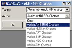
Figure 31. Assigning MM Charges with the Atom List Editor

This dialog is used to automatically assign charges to atoms for use in Molecular Mechanics calculations. The Target menu specifies which atoms should be assigned charges: all atoms, all selected atoms, or all atoms currently lacking an MM charge. The Action menu specifies which charge scheme should be used. Amber94 charges are always available. The other options in the list are available when they have been previously computed for the structure in a Gaussian calculation.

The View menu controls atom highlighting within view windows while the Atom List Editor is in use. Each item in the first section is a toggle, and check mark next to it within the menu indicates that it is enabled:

• Exclusive Highlighting: Only allow one row within the table to be highlighted. Clicking on the dot within the Highlight column deletes any current highlight.
• Z-Matrix Connectivity Highlighting: For each highlighted atom, also highlight the other atoms used to define its Z-matrix entry (i.e., bond, angle and dihedral specification).
• ONIOM Link Highlighting: Display atoms for which the highlighted atom functions as a link atom for ONIOM calculations (labeled in the View window with [Link]), based on the contents of the row’s ONIOM layer data.

The remaining items on the View menu have the following effects:

• Center Highlighted Atoms in View: Reposition the structure in the active View window so that highlighted atoms appear in the center.
• Select/Deselect Highlighted Atoms: Add/remove highlighted atoms from the current selection.
• Highlight Crowded Atoms: Turn on highlighting for atoms that are unphysically close to one another (within 0.75 Angstroms).

The Rows menu controls whether some or all atoms within the molecule are visible in the table and also provides some shortcuts for selecting groups of atoms:

• Sublist Filters: Open the Sublist Filters dialog for defining atom filter expressions (described below).
• Sort Selected: Sort highlighted atom list rows, according to the criterion selected in the submenu: Ascending by Highlight, or Descending by Highlight. The up and down arrow buttons in the toolbar are equivalent to these submenu items.
• Sublist: Toggle display of atoms in and/or not in the active sublist, depending on the submenu item that is chosen (Show Sublist Atoms or Show Non-Sublist Atoms). Current selections are indicated by a check mark next to the corresponding item on the submenu.
• Select All: Select all atoms unconditionally.
• Invert Selection: Deselect all currently selected atoms and select all deselected ones.
• Select Rows of Selected Atoms and Select Atoms of Selected Rows: Cause the selected atoms in the View and the selected rows in the table to be identical. The first of these gives priority to currently selected atoms, selecting corresponding table rows and deselecting others, while the second causes the View selection to match the rows selected within the table.

The Columns menu allows you to specify which columns appear in the table on an individual column basis. The first few items in the menu correspond to the default columns in the table, which are independent of the various column display buttons. The Freeze and Gaussian Fragment items further down in the list function in the same way.

You can select which columns appear for the Z-matrix Coordinates, Fractional Coordinates, ONIOM Layers, PDB Info, Isotope Masses and Molecular Mechanics Parameters buttons via the corresponding submenus. The Cartesian Coordinates item has the same function as the corresponding button although individual coordinates cannot be selected separately.

The Help menu item provides help for the Atom List Editor.

Using Sublist Filters

Sublist filters are a means of limiting the visible rows within the Atom List Editor to a manageable number for large molecules. They are defined by means of a dialog reached with the Atom List Editor’s Rows=>Sublist Filters menu path, illustrated in Figure 32.

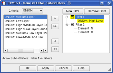
Figure 32. Creating Sublist Filters

This dialog allows you to create and apply sublist filters which are used to limit the rows which are displayed within the Atom List Editor. In this case, we apply two filters in succession: Filter 1 selects atoms in the High ONIOM layer and Filter 2 selects oxygen and nitrogen atoms within that subset.

To use the facility, you must first create a filter using the New Filter button. Filters are always named Filter n and cannot be renamed. The filter is defined using items from within the Criteria list; the popup menu displays the available categories of criteria items. In the figure, we are using the ONIOM category to define Filter 1. Select one or more criteria from the list and then use the > button to move them to the selected filter. Although we have not done so in the example, items from different Criteria categories can be combined with the same filter.

The >> button will similarly move all items within the list. Items can be removed from filters using the < and << items, to remove the selected item and all items (respectively). An entire filter is removed with the Remove Filter button.

Criteria within filters are combined with an OR logic: any atom matching any criterion will be displayed (or not, according to the settings on the Atom List Editor’s Rows=>Sublist submenu). Filters are activated and deactivated by selecting/deselecting the check box to the left of their name. When only a single filter is active, all atoms matching that filter are affected. When more than one filter is active, then all active filters are applied in series, in the order in which they are listed within the dialog, according to an AND logic. For example, Filter 2 is applied only to the matching atoms remaining after applying Filter 1. Subsequent filters will never enlarge the selection resulting from a previous filter, but rather only filter it further.

The available Criteria categories are:

• Tags: Select one or more atom tag numbers (serial numbers).
• Tag List: Select a list of atom tags.
• Elements: Select atoms by element type.
• ONIOM: Select atoms by ONIOM layer, layer boundary and/or link atom presence.
• MM: Select atoms having undefined Molecular Mechanics atoms types and/or MM charges.

Filters are specific to individual molecule groups, and they do not persist across different sessions for the corresponding input file. In other words, if you close and reopen the input file or if you exit and restart GaussView, current filters are lost.

Defining Isotope Masses and Isotopologues

The Atom List Editor provides an easy way for specifying alternate isotope masses for atoms which are relevant for some calculation types (e.g., vibration frequency analysis). By default, Gaussian assigns the most abundant isotope to each atom in a molecular structure. You can specify a different isotope by enabling the Isotope Masses button. Doing so will reveal a column titled Mass (Isotopologue 0). Each cell in the column contains a popup menu listing the possible isotopes for the element in that row of the table. You can select the desired isotope from the menu, or you may enter the desired value directly into the field. The Default choice always refers to the most abundant isotope.

You can define multiple isotopologues for the structure by adding additional columns to the table via the Columns=>Mass=>Mass (Isotopologue n) menu paths. These can be used for subsequent vibrational analysis visualization (discussed later).

The PDB Residue Editor and The PDB Secondary Structure Editor

Examining and modifying structures imported from PDB files may be made easier by the PDB Residue Editor and PDB Secondary Structure Editor, reached via the correspondingly named items on the Edit menu. They are illustrated in Figure 33.

The menus in these editors are very similar to those in the Atom List Editor discussed in the previous section. Briefly, they are:

• File: Contains items for exporting the data, printing the table and closing the editor.
• Edit: Contains items for undoing and redoing operations, copying data between rows, deleting all atoms or hydrogen atoms within selected residues/secondary structures, and adding hydrogens to the selected residues/secondary structures.
• View: Items allow you to enable/disable exclusive highlighting, center highlighted atoms in the View window, and select /deselect atoms within highlighted items.
• Rows: Allows you to sort the selected table rows and perform various selection operations.
• Columns: Used to show or hide various columns from the table.
• Help: Open the internal help related to the current editor.

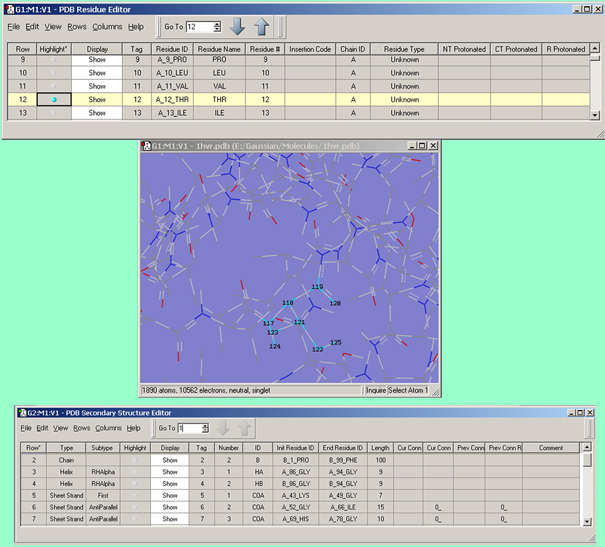
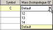
Figure 33. The PDB Residue and PDB Secondary Structure Editors

The PDB Residue Editor (top) and PDB Secondary Structure Editor provide mainly read-only views of residue and other data assigned in PDB files. The Display column can be used to hide the atoms in certain residues/secondary structures for easier viewing of the molecule’s key features. The Highlight column can be used to highlight the atoms corresponding to the selected item. In this example, we have highlighted residue 12 in chain A making it easy to locate in the View window below.

The Connection Editor

The Connection Editor, reached via the Edit=>Connection menu path, can be used to determine whether proper atom ordering is maintained throughout a molecule group. You can also use it to automatically reorder atoms to align atom tags between related structures across a molecule group (useful for preparing structures for QST2 and QST3 transition structure optimizations). Manual atom reordering is also possible.

When the Connection Editor is active, the molecule will be analyzed to determine if the atom tags match across the entire molecule group, and the status bar will report the result. If potentially fixable mismatches are detected, the dialog will report this and suggest that the user Enable Autofixing. Clicking on the corresponding button will tell the Connection Editor to reorder the atom labels to remove these mismatches. The success or failure of autofixing will be reported on the status bar. When autofixing is active, any manual reordering of atom tags will cause autofixing to be called and remove any mismatches that might have been introduced.

When active, autofixing can be disabled using the relabeled Disable Autofixing button. When autofixing is not applicable, the button is relabeled as No Autofixing.

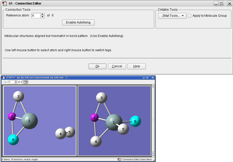
Figure 34. The Connection Editor

The Connection Editor is used to verify and assign atom equivalences in two molecular structures. When working with a molecule group, viewing in multi-geometry mode allows easier comparison and editing. In this contrived example, we need to swap the ordering of atoms 3 and 4 in one of the models in order for the atoms to correspond properly. This can be done by clicking on the Enable Autofixing button or via a manual process.

Atoms can also be manually reordered by using the mouse. These operations use a reference atom as their basis (see the first bullet):

• Left clicking: Designate the atom as the reference atom. This can also be done using the Reference Atom control.
• Middle clicking: Assign the tag one greater than the reference’s item to the selected atom.
• Right clicking: Swap tags with the atom and the reference atom. The atom then becomes the new reference atom.

The Apply to Molecule Group checkbox determines whether the Connection Editor’s actions apply only to the current model or to all models within the molecule group.

The ZMat Tools popup allows you to perform some Z-matrix operations on the molecule or molecule group:

• Sort H: Move hydrogen atoms to the end of the atom ordering.
• Reorder: Reapply standard Z-matrix ordering.
• Reconnect: Regenerate connectivity data.

The other items on this popup menu do not apply to Gaussian.

The Redundant Coordinate Editor

The Redundant Coordinate Editor allows you to create and edit redundant coordinates for use with Gaussian optimizations or potential energy surface scans. It is accessed via the Edit=>Redundant Coordinates menu path or the Redundant Coordinate Editor button. It is illustrated in Figure 35.

The central feature of this dialog is a scrollable list containing information on each of the coordinates. A pencil icon in the status column marks that coordinate as the currently active coordinate. A warning sign in the status column indicates that that coordinate is incomplete or invalid. When the currently active coordinate is invalid or incomplete, the status bar at the bottom describes the nature of the warning. The coordinate column contains a brief description of the coordinate and its parameters.

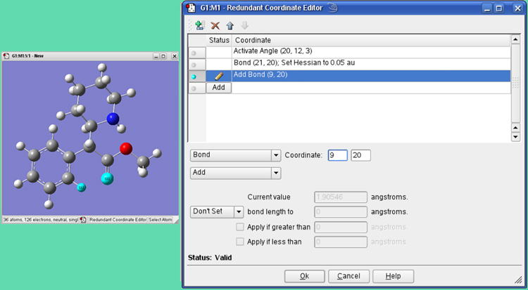
Figure 35. The Redundant Coordinate Editor

We are adding the bond coordinates for the two selected atoms so that its distance will be reported in the optimization output (even though the atoms are not in fact bonded to one another). The list in the window also shows 2 other coordinates we added.

A toolbar at the top provides buttons for adding a new coordinate, deleting a coordinate, and moving an item up or down in the list. Adding a new coordinate creates an unidentified coordinate, which is placed in the list just after the currently active coordinate and becomes the active coordinate.

All of the available redundant internal coordinate types are supported by the various selections in the two popups in the Coordinate area, and the items on these menus are self-explanatory. Any additional fields required by a specific coordinate type will appear in the panel when the type is selected. See the discussion of Opt=ModRedundant in the Gaussian 09 User’s Reference for more information. The Set/Don’t Set popup and related fields allow you to specify the value of a coordinate or an increment to its current value.

When exiting the Redundant Coordinate Editor, if any coordinates are still invalid or incomplete, you will be notified and given the option of continuing to edit. If you exit anyway, any invalid coordinates will be deleted.

Specifying ONIOM Layers

Choosing the Edit=>Select Layer menu item or clicking on the Select Layer button opens the Layer Selection Tool. This window is used to assign atoms to ONIOM layers graphically. It is illustrated in Figure 36.

There are several methods for selecting atoms for layer assignment:

• You can use one of the buttons at the top of the dialog. The All button selects all atoms in the molecule, and the None button deselects all atoms. The Layer button selects all atoms currently assigned to the specified layer. The Select PDB Residues opens another selection dialog which allows you to select atoms by residue if this information was present in the PDB file corresponding to the current model (see Figure 37 below).
• Use the left mouse button to select or deselect atoms manually, continuing until all the atoms that you want have been selected. Hold down the Shift key to add to the current selection.
• Proximity-based selection: Select an atom, and then use the Expand Selection slider and proceed until you have selected all the atoms you need. Moving it to the right increases the distance used when selecting atoms.

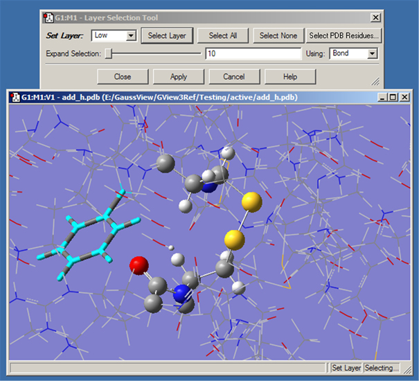
Figure 36. Assigning Atoms to ONIOM Layers

This dialog allows you to assign atoms to layers for ONIOM calculations. Different layers are indicated by the different display formats. Here, the atoms in the ring at the left are selected for layer assignment.

For distance based atom selection, the distance between atoms to be selected depends on the following criteria, selected in the Using popup menu:

• Bond, which selects only atoms that are bonded.
• Distance, which selects an atom based solely on proximity to a current selection, regardless of whether or not it is bonded.

Layer Selection by PDB Residue

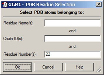
Figure 37. Selecting Atoms for Layer Assignment by PDB Residue

This dialog allows you to specify the desired residue by residue name (type), residue number and/or chain (A or B). Omitted items act as wildcards. For example, if you enter only residue number 22, then residue 22 in both chains will be selected. Similarly, entering only a residue name will cause all residues of that type within the molecule to be selected.

Confirming Layer Assignments

Once atoms are selected, you must click on the Apply button to assign them to that layer. Note that clicking on Apply turns off the selection. If you close the panel without applying your changes, they will be lost.

Layer Display Formats

By default, atoms in different layers are displayed in different formats in the View window. Using the standard settings, atoms in the High layer appear in ball-and-stick format, atoms in the Medium layer are displayed as tubes, and atoms in the Low layer are in wireframe format. These can be customized with View=>Display Format for the current molecule or, for all future views, via the corresponding fields in the Molecule panel of the Display Format Preferences.

The Molecular Orbital (MO) Editor

The Edit=>MOs menu path and the MO Editor button both open the MOs window, illustrated in Figure 32. It is used to inspect molecular orbitals (MOs) from Gaussian calculations—MO energy and occupancy diagrams, visualized MO isovalue surfaces—as well as to quickly generate new MOs and/or visually select active-space MOs to be used for CASSCF calculations.

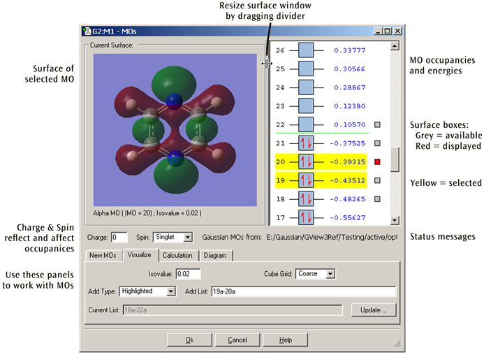
Figure 38. The MO Editor

This window is used for examining molecular orbitals visually and potentially rearranging their occupancies and/or ordering for a subsequent Gaussian calculation. Here we are viewing MO 20, one of 5 available surfaces (and 2 selected MOs).

The MOs dialog has its own embedded View window for displaying the molecule and surface corresponding to the currently selected MO (if available). This embedded view is read-only and cannot be used to edit the molecule. In viewing functionality, it functions almost identically to a standard View window in terms of includes keyboard and mouse controls for translating, rotating, and zooming the molecule, accessing the context menu, and so on. (See the discussion of manipulating views earlier in this chapter and that concerning surfaces in “Viewing Gaussian Results” for details.)

The size of the Current Surface window can be changed by resizing the entire MOs dialog. Its width can also be adjusted by clicking and dragging on the partition between it and the MO diagram. This adjusts the relative widths of the two windows.

MOs can be selected for visualization, inclusion in future calculation, and other operations by left-clicking on them. Selected MOs are highlighted in yellow. If a surface is available for an MO, a small square appears to the right of the MO. The square is red for the MO whose surface is currently being viewed. Clicking on a different MO’s grey square will change the Current Surface View to show that MO’s surface.

The bottom portion of the window contains four panels:

• The New MOs panel is used to read-in or generate molecular orbitals.
• The Visualize panel allows you to generate surfaces for desired MOs.
• The Calculation panel allows you to modify the order of MOs for future Gaussian jobs.
• The Diagram panel controls the energy level and orbital occupancy display to the right of the view area.

The Visualize panel is visible in Figure 39. The various fields in it specify which orbitals should be visualized, along with two surface generation parameters (the isodensity value and the grid density, via the Isovalue and Cube Grid fields, respectively). The Add Type popup contains items which specify which MOs to visualize; its options are generally self-explanatory with the possible exception of Current List (regenerates the orbitals listed in the Current List field) and Other (specifies the arbitrary list of orbitals present in the editable Add List field). Note that GaussView attempts to keep the Add List and Add Type fields synchronized. Clicking the Update button will generate the requested orbital surfaces.

Figure 39 displays the other panels present in the MO Editor (stacked on top of one another), each of which will be discussed in the course of the remainder of this section.

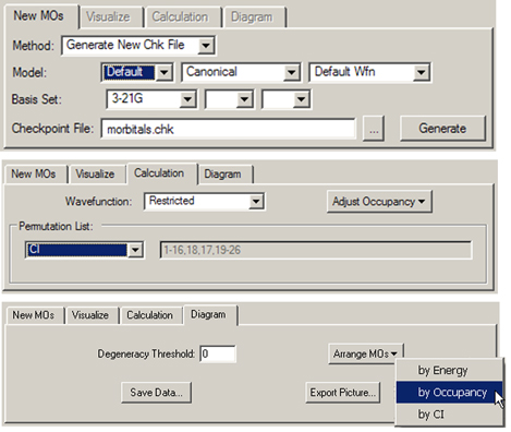
Figure 39. The MO Editor’s New, Calculation and Diagram Panels

Each panel shows a typical use for it (and not necessarily the default settings).

Modifying Orbital Occupancies, Molecular Charge and Spin Multiplicity

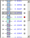
To the right of the Current Surface is the MO energy and occupancy diagram showing the MOs for the current molecule if available, initially arranged in order of increasing energy. Alpha and Beta electrons are represented by red up and down arrows in a blue box, respectively. Electrons can be moved from one MO to another by dragging them between the corresponding boxes. Electrons can also be added or removed from an MO by right-clicking in the MO box. Manipulating the MO occupancies in this way changes the net charge and/or spin multiplicity of the molecule as appropriate, reflected in the Charge and Spin fields. These fields can also be edited directly, and any changes will be reflected in the MO occupancies. Increasing the charge will remove electrons from the MOs, starting with the HOMO. Decreasing the charge will add electrons to the MOs, starting with the LUMO (or the HOMO if it is singly occupied). Similarly, increasing the spin multiplicity will move electrons from the highest doubly occupied MOs to the lowest virtual MOs, and decreasing the spin multiplicity will move electrons from the lowest-energy singly occupied MOs to the highest-energy singly occupied MOs. Finally, modifying the charge will also affect the spin multiplicity if the charge is changed by an odd number.

Controls in the Calculation panel also serve this purpose. The Adjust Occupancies popup contains two choices:

• Aufbau: Fill MOs with electrons in order of increasing orbital energy, in keeping with the current settings of Charge, Spin, and Wavefunction.
• Original: Restore the original read-in or computed orbital occupancies, modifying the Charge, Spin, and/or Wavefunction if appropriate.

Controlling the Orbitals Display

The Diagram panel controls the orbital diagram. The Arrange MOs popup allows you to order orbitals by increasing energy, by occupancy, or by CI; the latter is appropriate for creating a CAS active space (see below). The Degeneracy Threshold sets the value below which to consider orbital energies as equal. This feature is illustrated in Figure 40.

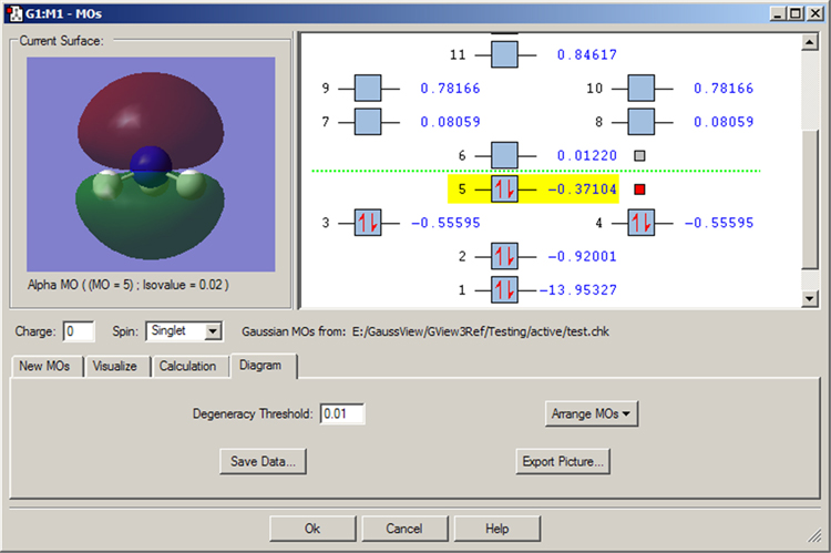
Figure 40. Degenerate Orbitals in the MO Editor

This MO display for NH3 illustrates how degenerate orbitals appear in the orbital display area. Note that we have modified the Degeneracy Threshold from its default value of 0 to allow GaussView to detect the degenerate MOs.

Generating and Retrieving MOs

The New MOs panel allows you to read-in or generate MO data, depending on the setting of the Method popup. When it is set to Load Existing Chk File, you can read in orbital data from a checkpoint file by specifying its location and then clicking Load.

When Method is set to Generate New Chk File, the Model and Basis Set areas specify the calculation model for generating orbitals. The fields labeled Model specify the initial guess type, localization method and wavefunction type, while the desired basis set is specified in the fields below these. The fields in the second line of this panel specify the basis set to use for the Gaussian calculation. Consult the discussion of the Guess keyword in the Gaussian 09 User’s Reference for more information on the various fields and choices. Clicking Generate will launch a Gaussian job to generate the orbital data (calculation type is Guess=Only).

Rearranging Orbital Ordering

The Permutation List control in the Calculation panel displays the current orbital reordering at any given moment; it is initially empty. The popup in this area offers three choices for orbital reordering:

• Occupancy (Alpha): Reorder orbitals based on the current occupancies of the alpha orbitals. This will order filled orbitals below unfilled ones, and fully occupied orbitals below partially occupied ones. Within each group, orbitals are arranged according to increasing energy.
• Occupancy (Beta): Reorder orbitals based on the current beta orbital occupancies (as in the previous item). Only available for unrestricted wavefunctions.
• CI: Reorder orbitals so that all occupied and all unoccupied orbitals are contiguous, with each group arranged in increasing energy order. This choice is appropriate for a CAS calculation.

Miscellaneous Options

The Diagram panel contains two additional controls:

• Save Data: Save the molecular orbital information from the MO diagram to a simple text file: orbital number, occupancy, orbital energy for each orbital and the number of frozen orbitals. For unrestricted wavefunctions, alpha and beta information will be saved in separate blocks.
• Export Picture: Save a graphic image of the MO diagram. You will be prompted for the filename and desired graphics format.

Building Periodic Systems with the Crystal Editor

The Edit=>PBC menu path and the Crystal Editor button both bring up the PBC window. This tool is used to specify unit cells for periodic systems. In order to use this feature, as well as to perform Periodic Boundary Conditions calculations in Gaussian, you will need some understanding of periodic systems, space groups, and general related terminology. This background is assumed in this section.

The window contains five panels:

• Symmetry: Specifies the dimensionality of the unit cell, the lattice system and space group constraints.
• Cell: Specifies dimensions of the unit cell and contains controls for repositioning & reducing cell contents.
• View: Specifies how many cells are displayed in each direction in the View window, as well as controlling the display/non-display of various items.
• Contents: Contains a list of atoms in the cell as an embedded mini Atom List Editor. Its popup also allows you to modify bonding.
• Reduce: Allows you to reduce the dimensionality of a unit cell (e.g., from a 3D system to a surface).

From the highest-level view, a typical process of building a periodic system might proceed as follows (consult the PBC tutorials in the GaussView online help for more detailed instructions):

[1] Use the Symmetry panel to specify the number of dimensions and desired space group.

[2] Add atoms to the cell using the mouse or via the Contents panel.

[3] Remove any unwanted atoms (e.g., if you used a fragment as a shortcut to creating the necessary atoms).

[4] Set the unit cell size using the Cell panel.

[5] Adjust bonding using the Contents panel if appropriate.

[6] Reduce cell contents if appropriate.

[7] Specify display properties using the View panel as desired.

The controls in each of the PBC window panels will be described in turn in the following subsections.

The Symmetry Panel

The Symmetry panel is displayed in Figure 41. It contains the following controls:

• Lattice Dimensions: Sets the number of dimensions in which the system has translational symmetry (i.e., is periodic): One for polymers, where a is the translation vector; Two for sheets, where a and b are the translation vectors, and Three for crystals, where a, b and c are the translation vectors.
  
  Note that the dimensionality of a lattice is not necessarily the same as the dimensionality of the corresponding cell contents. For example, the monomers of a polymer (a one-dimensional lattice) are generally not linear.
• Minimum Lattice System: 3D cell changes are constrained to preserve the specified lattice system. This control is read-only in the current version of GaussView (contrary to some earlier version).
• Enable Space Group Symmetry: Monitor space group symmetry and enforce space group symmetry constraints.
• Always Track Space Group Symmetry: Monitor space group symmetry during interactive changes to cell contents (e.g., continuously as the bond length slider is used) instead of only computing it after the change is completed.

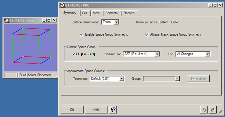
Figure 41. The PBC Symmetry Panel

This panel shows settings for a 3D periodic system constrained to the indicated space group.

These controls appear in the Current Space Group panel:

• Constrain To: Constrain changes to preserve at least the specified space group. All space groups to which the system exactly belongs are available for constraint.
• For: Enforce space group symmetry constraints for at least the specified type(s) of changes. Cell Changes refers to changes in the cell lengths or angles. Contents Changes refers to changes in the numbers, types and/or positions of atoms and bonds. The default is All Changes (i.e., both).

These controls appear in the Approximate Space Groups area of the panel:

• Tolerance: Set the tolerance for approximately belonging to a space group, in fractional coordinates. A selection can be made from the list or you can enter any value you want into this field. Valid input consists of any floating point number (e.g., 0.25) or fraction (e.g., 1/4).
• Group: Set the space group to exactly symmetrize to when the Symmetrize button is pushed. All applicable space groups within the specified tolerance are listed.

The Symmetrize button will symmetrize the system to exactly belong to the specified space group.

The Contents Panel

The Contents panel contains an embedded mini Atom List Editor which functions like the corresponding tool. It is illustrated in Figure 42. The controls at the top of the panel are:

• Intercell Coordinate Changes: Specify how to handle intercell coordinate changes. The selections are Fix Contents’ Cartesian Coordinates, Fix Contents’ Fractional Coordinates, and Fix Cell Parameters.
• Bonds: Recalculate or remove intracell and/or intercell bonds. Rebonding is based on distance criteria. The various selections on this menu are shown in Figure 42.

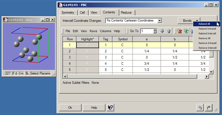
Figure 42. The PBC Contents Panel

This panel displays an atom list for the contents of the unit cell. It also contains the Bonds button which allows you to rebond atoms as appropriate, typically after modify parameters with the Cell panel (see Figure 43).

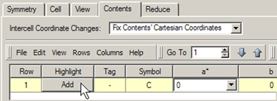
Adding atoms with this panel uses a procedure similar to that with the Atom List Editor. There is an Add button in the final row of the table (row 1 when the table is empty). In order to activate it, you must enter an element type into the column. You can also use the remaining columns to specify the fractional coordinates for the new atom. Note that additional atoms will also be added when you click Add in order to conform to space group constraints.

The Cell Panel

The Cell panel is displayed in Figure 43.

The Cell Changes popup specifies what should happen to the cell contents when the cell parameters are changed. When Fix Contents’ Cartesian Coordinates is selected, the contents of the cell and their Cartesian coordinates after a change are the same as before the change, provided the atoms are still within the cell boundaries.

The setting of the Add/Remove Atoms checkbox affects the operation of this choice:

• If unchecked, the contents of the cell and their Cartesian coordinates after a change are the same as before the change. For example, if there is one atom in the cell with fractional coordinates (1/2, 1/2, 1/2), and the length of a is doubled, the contents of the cell after the change will still be one atom, but with fractional coordinates (1/4, 1/2, 1/2).
• If checked, the contents of the cell after a change is defined as whatever atoms are within the cell boundaries after the change. For example, if there is one atom in the cell with fractional coordinates (1/2, 1/2, 1/2) and the length of a is doubled, the contents of the cell after the change will be two atoms, with fractional coordinates (1/4, 1/2, 1/2) and (3/4, 1/2, 1/2).

When Cell Changes is set to Fix Contents’ Fractional Coordinates, the contents of the cell and their fractional coordinates after a change are the same as before the change. For example, if there is one atom in the cell with fractional coordinates (1/2, 1/2, 1/2) and the length of a is then doubled, the contents of the cell will still be one atom with fractional coordinates (1/2, 1/2, 1/2). This option is often the more useful of the two.

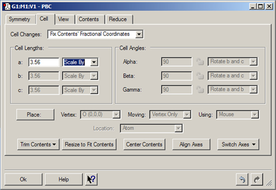
Figure 43. The PBC Cell Panel

This panel is being used to resize the unit cell. The values in the disabled fields are predetermined by the space group to which the structure is constrained (see the Symmetry panel in Figure 35).

The controls in the Cell Lengths and Cell Angles areas control the geometry of the cell:

• a, b, c: Set the length (in Angstroms) of the indicated cell vector.
• Scale by: Scale the length of the cell vector by a positive number.
• Alpha, Beta, Gamma: Set the angle (in degrees) between the other cell axes (i.e., between the b and c cell axes for the Alpha field). The specified angle is changed by rotating one or both of the other two cell axes, as specified in the corresponding Rotate field. Even for non-orthogonal cells, the rotation(s) used to change an angle are constrained to not change the other two angles.
• Padlock icon: If locked, freeze the specified angle at its current value. The angle is also constrained to its current value during vertex placement.
• Rotate: Specify the axes to rotate when the specified angle is changed. You have the choice of selecting either one or both of the other two axes.

Figure 44 illustrates the GaAs unit cell we are working on after specifying cell lengths as in Figure 43 and then rebonding in the Contents panel (see Figure 42).

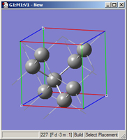
Figure 44. Modified and Rebonded GaAS Unit Cell

View appearance after the operations in Figures 42 and 43.

The fields in the next two rows of the panel control placement of the cell vertices (which define the boundaries of the unit cell):

• Place: Enable/disable cell vertex placement.
• Vertex: Specify the cell vertex to be placed.
• Moving: Specify whether to move the vertex only or move the whole cell.
• Using: Specify whether to place the vertex using mouse selection in the View window or fractional coordinates.
• When Using is set to Mouse, the popup specifies the location type for vertex placement using mouse selection in the View window, Atom means that the vertex will be placed on the atom you click on, Between Two Atoms means that the vertex will be placed midway between the two atoms you click with the mouse, and Any Point means that the vertex will be placed at the point in space where you click.
• When Using is set to Coordinates, additional fields appear for the desired fractional coordinates. Click the Apply button to place the vertex at the specified coordinates.

The five buttons at the bottom of the panel have the following purposes (the examples use a 3D cell):

• Trim Contents: Change the cell contents using the specified method. If Delete All Atoms Outside Cell is selected, then all atoms outside the cell boundary are deleted. If Translate All Atoms Inside Cell is selected, then all atoms outside the cell boundary are translated to the equivalent position inside the cell boundary. Redundant atoms are deleted. An atom is considered outside the cell boundary if one or more of its fractional coordinates is less than zero or greater than or equal to one.
• Resize to Fit Contents: Change the cell lengths to fit the cell contents, then center the contents. A 0.5 Angstrom cushion is added to each side of the cell.
• Center Contents: Translate the cell so that its center (1/2, 1/2, 1/2) coincides with the contents’ center of nuclear charge.
• Align Axes: Align the Cartesian origin and axes with those of the cell. The cell origin (0,0,0) is first translated to the Cartesian origin. The cell is then orthogonally rotated so that the c cell axis is aligned with the Cartesian Z-axis. The cell is then orthogonally rotated so that the a cell axis is aligned with the Cartesian Y-axis. The cell is then orthogonally rotated so that the b cell axis is aligned with the Cartesian X-axis.
• Switch Axes: Switch the specified pair of cell axes. For example, if a <–> b is selected, then the a vector becomes the b vector and vice-versa.

The Reduce Panel

The Reduce panel is displayed in Figure 45. It contains the following controls:

• h, k , l: Set the Miller index for the reduced lattice intercept along the a, b or c axis (respectively).
• n(h), n(k), n(l): Set the multiple for the reduced lattice intercept along the a, b or c axis.
• Highlight Reduced Lattice Plane: Indicate the pending reduced lattice in the View window (see Figure 45).
• Reduce Lattice: Reduce the lattice by one dimension according to the specified Miller parameters.

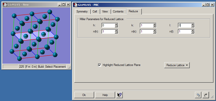
Figure 45. The PBC Reduce Panel

This panel is used to convert a unit cell to one having a lower dimensionality. Here, we are reducing a palladium 3D cell to a surface two atoms deep. The light colored plane indicates the cut.

The View Panel

The View panel is displayed in Figure 46. It contains the following controls:

• a, b, c, -a, -b, -c: Set the number of cells to display along the specified axis (in the positive or negative direction, as indicated). This number is for display purposes only; it does not change the contents of the unit cell unless the Combine button is pushed. See Figure 46.
• Combine: Combine all of the displayed cells into one larger “supercell.”
• Show Reference Cell Edges: Display cell edges and vertices of the reference cell.
• Show Replicate Cell Edges: Display cell edges and vertices of all replicate cells.
• Show All Boundary Atoms: Display all atoms on cell boundaries.
• View Along: Align the specified Cartesian or cell axis of the system with the axis perpendicular to the plane of the computer monitor.
• Replicate Contents Display: Specify how the atoms and bonds in replicate cells should be displayed. The choices include a normal display, a dulled-out normal display, the display format defined for one of the ONIOM layers in the Molecule panel of the Display Format Preferences, or no display.
• General Positions: List of equivalent positions (in fractional coordinates) for the current (constraint) space group. The Display popup specifies how to view the asymmetric units corresponding to the general positions for the current (constraint) space group.
• Special Positions: List of special positions (in fractional coordinates) for the current (constraint) space group. The Display popup specifies how to view the special positions for the current (constraint) space group.

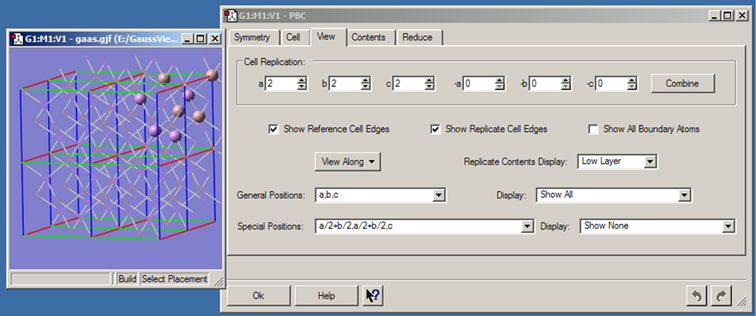
Figure 46. The PBC View Panel

This panel specifies how many unit cells appear in the View window. The View window shows a 3D gallium arsenide structure. Two cells in each direction are displayed. The contents of replicate cells are displayed using the Low Layer display format (their default display mode).

Specifying Fragment Placement Behavior

The small triangle above the Current Fragment area of the GaussView control window can be clicked to reveal some advanced options to specify how new fragments are joined to an existing molecular structure. The Mode popup allows you to select the settings (in which case, all fields are disabled), to specify Custom settings, or to restore the previously-used (Old) non-default settings (also nonmodifiable). You must select Custom in order to make changes to these items. The values for these three groups of settings can be specified in the Building Preferences.

There are two panels in this area. The Before panel, pictured in Figure 47, sets restrictions for how fragments may be added to a structure. The After panel (see Figure 48) specifies how the structure is treated after a fragment is added.

Here are some preliminary definitions necessary for understanding the options in these panels:

• The target atom is the one selected with a mouse click.
• The hot atom is the atom in the new fragment that takes the place of the existing target atom when the two pieces are joined.
• A terminal atom is any atom bonded to only one atom.
• A terminal valence atom is a hydrogen atom or an open valence bonded to only one atom.
• A join-bond is a bond between the hot atom and any terminal atom. These are bonds that can be eliminated in the process of connecting the fragment to the target atom. When a fragment is joined to the target atom, there must be one join bond in the fragment for each corresponding bond to the target atom.

These are the items in the Fragment Placement Before panel:

• Target and Fragment Join-Bond Types Must Match: The selected join-bonds in the fragment must match the bond types of the target atom. Enabling this item will prevent many placements.
• Fragment Join-Bonds Can Be Any Terminal Bonds: Normally, only hydrogen or open valences are taken as join-bonds. When this option is on, any terminal atoms are also candidates for join-bonds. For example, the oxygen atom in formaldehyde could be used as a join-bond for ethylene because the bond type matches (double bond).

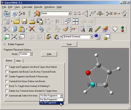
Figure 47. Fragment Placement Restrictions

The items in this window set restrictions on the circumstances in which fragments may be joined to an existing structure. This window shows the default values.

• Create Fragment Join-Bonds If Necessary: This option will allow most fragments to be attached to any target. If the fragment does not have enough join-bonds for a given target selection, additional valences will be added to satisfy the requirement. Again, the join-bonds are deleted when fragment and target are joined as well as the target atom (on by default).
• Terminal Hot Atoms Define Join-Bonds: This option makes it easier to choose terminal atoms as hot atoms. Since most terminal atoms have no join-bonds, the option will use the one bond as the join-bond. However, the bond will not be deleted. This is useful when you have a central atom with more than one terminal bond, and you want to explicitly choose which terminal bond will be used to do the joining.
• Bond to Target Atom Instead of Deleting It. This option allows you to bond the fragment to target atom itself, deleting only the join-bonds.
• Delete Any Terminal Atoms Bonded to Target Atom: Remove extra terminal bonds.
• Automatically Select Hot Atom: This item is designed for use with biological fragments (which is its default setting). It causes GaussView to determine the hot atom dynamically. This makes it easier to build amino acid residues, etc., by producing a sensible backbone as you add residues.

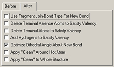
Figure 48. Structure Options After a Fragment Placement

The options in this panel allow you to select actions for GaussView to perform automatically after a fragment is added to a molecular structure. The settings in this example are the defaults.

These are the items in the After panel:

• Use Fragment Join-Bond Type For New Bond: Normally, the bond connecting the fragment to the target bond type is determined by the original target bond. If this option is on, the fragment’s bond type is used instead. This option is useful when the Match Bond Types option is off.

The next three items activate electron bookkeeping at the target atom site. Note, however, that non-terminal atoms are not affected. Also, GaussView does not reduce or elevate the bond type to satisfy valency requirements.

• Delete Terminal Valence Atoms to Satisfy Valency: Allows terminal valence atoms to be deleted to reduce overloaded valency at the target atom site.
• Delete Terminal Atoms to Satisfy Valency: Allows for any terminal atom to be deleted to reduce overloaded valency.
• Add Hydrogens to Satisfy Valency: Automatically adds hydrogen atoms to satisfy valency requirements.

The remaining options enable automatic cleaning operations, and they are self-explanatory: Optimize Dihedral Angle About New Bond, Apply “Clean” Around Hot Atoms, and Apply “Clean” to Whole Structure.