Viewing Gaussian Results
This section describes the Results menu and the options available through it. This menu opens a series of dialog boxes that allow you to examine the results of calculations from Gaussian output files. If the selected item is not present in the file, the item is dimmed in the menu.
The various spectra and plots produced by GaussView can all be customized and manipulated using common techniques. These procedures are discussed in the final part of this section of the manual.
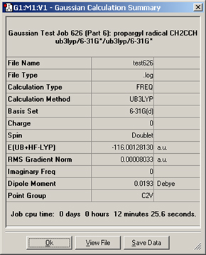
The Results=>Summary menu item displays summary data about the results of the Gaussian calculation (available when a Gaussian log file or checkpoint file is opened). It is displayed in Figure 83.
Figure 83. Summary of a Gaussian Calculation
This window summarizes the results of a B3LYP/6-31G(d) frequency calculation.
The Results=>View File menu item and the button can both be used to open the Gaussian log file associated with the Gaussian calculation (if applicable).
![]() The Results=>Stream Output File menu item and the button can both be used to view the Gaussian log file associated with the current Gaussian calculation continuously as the job runs.
The Results=>Stream Output File menu item and the button can both be used to view the Gaussian log file associated with the current Gaussian calculation continuously as the job runs.
Displaying Atomic Charges Computed in Gaussian
The Results=>Charge Distribution menu item opens the Display Atomic Charges dialog (see Figure 84). This tool manages the display of partial charge density as computed by various methods in Gaussian. Displays are available for the default Mulliken charges and other computed charges that are available for this job. The Charge Type menu lists the available choices.
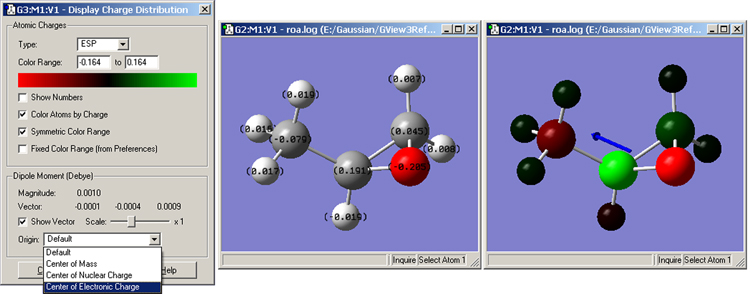
Figure 84. Displaying Atomic Charges
The dialog on the left is used to control what charges are shown and how they are displayed. The window in the middle shows the numeric charge numbers display, and the one on the right shows the atoms colored by charge (reflecting the settings in the dialog on the left), as well as the dipole moment vector.
By default, the color spectrum for charge display is set by reading the maximum charge computed for the molecule and setting the range to match the charge. The range can also be adjusted manually by entering values into the Charge Range fields.
The remaining checkboxes in the top portion of this dialog have the following meanings:
The Dipole Moment area of the dialog controls whether a vector representing the dipole moment is included in the display. When the vector is displayed, you can specify the scaling factor for the vector’s length (the default is about 1.0) as well as its origin.
The buttons at the bottom of the Display Charge Distribution dialog control whether the display persists after the dialog is closed. Clicking will cause the atomic charges display to be retained, while clicking will return the View window to its normal state.
Charge Distribution Preferences
Defaults for the items in the Display Atomic Charges dialog can be set with the Charge Distribution Preferences panel (see Figure 85).
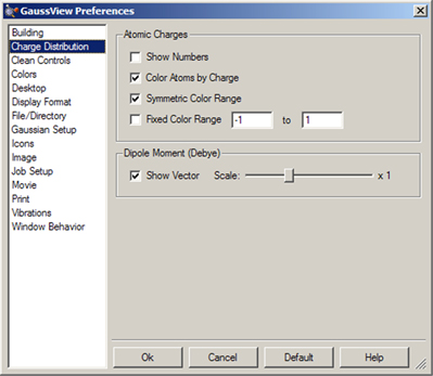
Figure 85. Charge Distribution Preferences
This preference panel specifies how atomic charge results are visualized, using the same options as in the Charge Distribution dialog.
Displaying Surfaces and Contours
The Results=>Surfaces/Contours menu item opens the GaussView Surfaces and Contours dialog (see Figure 86). It allows you to display various chemical data in three dimensions. The surface data may be generated from a Gaussian checkpoint file or be read in from a cube file. Note that there are two steps involved in actually displaying a surface:
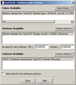
Figure 86. The Surfaces and Contours Dialog
This dialog allows you to select cubes for display as surfaces and/or contours and also to manipulate currently displayed surfaces and contours.
Generating and Manipulating Cubes
The following items in the Surfaces and Contours dialog relate to cubes:
The New Cube selection on the Cube Action button’s menu brings up the dialog in Figure 87. It is used to generate new cubes from the electron density and other data in the checkpoint file. GaussView automatically invokes the CubeGen utility.
The Type popup selects the molecular property for which to generate a cube. For most selections, additional fields will appear to further specify the desired data. For example, in Figure 87, the density matrix to use when generating the electrostatic potential cube can be selected. Similarly, for molecular orbitals, the specific orbital(s) to generate are indicated via additional fields.
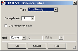
Figure 87. The Generate Cubes Dialog
This dialog will generate the type of cube specified in the Type field. Here, we are generating a cube of the electrostatic potential computed from the SCF electron density (frozen core by default).
The Grid field is used to specify the density of the cube. Increased density brings increased computational requirements. Generally, the default setting of Coarse is adequate for most visualization purposes, Medium is adequate for most printing and presentation purposes. The equivalent number of points per “side” is indicated in the second field in this line for each of the Coarse, Medium and Fine selections. Use the Custom item to specify a different value.
Clicking the button will generate the cube (as a background calculation) and exit the dialog. The new cube will appear in the Cubes Available list when the calculation finishes. You can view the job via the Calculate=>Current Jobs menu item or the equivalent button. Note: Cubes generated on the fly in this manner are not saved to disk unless you do so explicitly; otherwise, they will be lost when GaussView terminates.
There are several items in the Type popup that allow you to transform one or more cubes: you can scale and square cubes and add or subtract two cubes. For example, if you wanted to display a difference density, you can load in the two cube files (e.g., the densities computed in the gas phase and in solution). Once they are loaded, you can create a new cube (via Cube Actions=>New Cube) and then select Subtract Two Cubes from the Type menu.
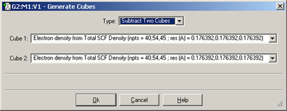
Figure 88. Creating a Cube as the Difference of Two Densities
This dialog creates a new cube that is the difference between corresponding values in the two source cubes.
The following items in the Surfaces and Contours dialog relate to surfaces:
The Surface Actions menu includes these items:
Figure 89 shows some example surfaces.
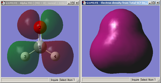
Figure 89. Example GaussView Surfaces
These windows display the HOMO molecular orbital surface (left, displayed in transparent mode) and an electron density surface (right, displayed in solid mode). Both are for formaldehyde.
Note that surfaces cannot be saved as data (only cubes can). Rather, they must be recomputed when they are desired. Images of surfaces can also be saved as image files for use in other contexts.
GaussView also allows you to map the values of one property on an isosurface of a different property. This is accomplished by selecting the New Mapped Surface item from the Surface Actions button’s menu. This will bring up the dialog illustrated in Figure 90.
The fields in this dialog have the following purposes:
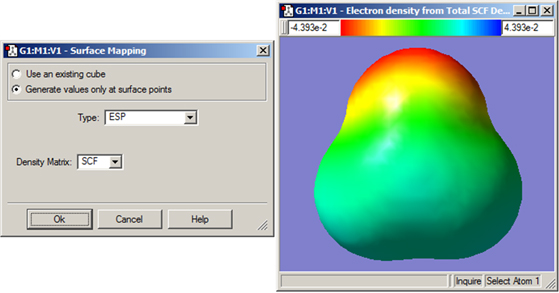
Figure 90. Creating a Mapped Surface
This dialog allows you to create a surface in which the coloring is determined by the values of a second property. The window on the right shows an electron density surface painted according to the value of the electrostatic potential for formaldehyde.
View windows display mapped surfaces and include a color mapping toolbar at the top (as in the window on the right in Figure 90). The colors used in rendering a mapped surface are based on a uniform scaling between minimum and maximum values, as specified in the text boxes to the left and right of the spectrum (respectively). Changing the values in these boxes will change the color scale and correspondingly change the coloring on the mapped surface. Like other toolbars, this color mapping toolbar can be moved around the edges by simply clicking and holding on the grip bar and dragging around the window.
Surfaces may be displayed in solid, transparent and wire mesh forms. The surface display may be modified using the Display Format dialog’s Surface panel (accessed via the View=>Display Format menu item and the equivalent button on the toolbar). The dialog format for a transparent surface is displayed in Figure 91.
The Z-Clip slider is present in the dialog for all three surface types. It may be used to remove the frontmost portions of the image to allow views into the interior of the molecular display.
The IsoValues popup controls whether the positive values, negative values or both (the default) are displayed. The Hide backside checkbox controls whether the back side of surfaces are displayed. Checking it results in increased transparency for transparent surfaces. Try turning it on and off with the Format set to Mesh to see exactly what is being hidden or revealed.
Defaults for surface properties can also be set via the Display Format Preferences’ Surface panel, which contains the same controls as in Figure 91.
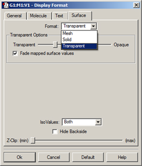
Figure 91. Customizing a Surface Display
This dialog allows you to modify the display of surfaces. Here, we are setting the properties of a transparent surface. The Transparent Options slider varies the opacity of the transparent surface. The Fade mapped surface value checkbox causes the values in the midrange of the spectrum to become transparent (i.e., those close to zero).
Contours are two dimension projections of cube data into a plane. They also use the cubes generated in the Surfaces and Contours dialog (see Figure 86). The items on the Contour Actions menu work analogously to those on the Surface Actions menu: you can use them to create a new contour (New Contour), to display or hide a contour (Show Contour and Hide Contour) and to remove a contour (Remove Contour). Figure 92 illustrates an example contour display.
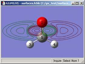
Figure 92. Example Contour Plot
This contour projects the HOMO into a plane perpendicular to the C=O bond.
Figure 93 illustrates the dialog that results from selecting Contour Actions=>New Contour. It contains four subareas:
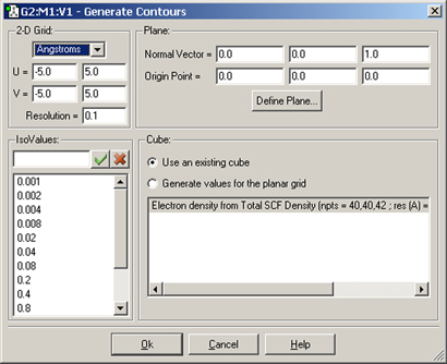
Figure 93. The Generate Contours Dialog
This dialog will generate a contour from an existing cube created or loaded previously via the Cube Actions menu in the Surfaces and Contours dialog.
By default, the contour plane is defined as the view’s XY plane. The plane can be defined in the Contour dialog’s Plane area. It is defined as the plane perpendicular to the vector defined by the specified Normal and Origin points in the dialog. The default origin point is (0,0,0) and the default point defining the normal vector is (0,0,1).
More complex plane definitions can be specified by clicking on the button, which brings up the dialog in Figure 94. There are two methods for defining the plane: Normal Vector (as described above) and Three Points (illustrated in the figure). In the latter method, you define the origin and two other points to define the contour plane (traditionally referred to as O, P and Q). The easiest way to define the points is to specify atoms for them, but you can also enter lists of atoms (the average of their coordinates will then be used) or completely arbitrary Cartesian coordinates.
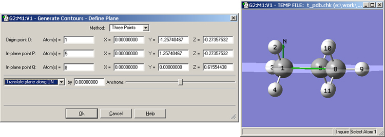
Figure 94. Specifying the Desired Contour Plane
In this example we are defining the contour plane as the one containing the carbon atoms, using the 3 points definition method. The green lines in the View window indicate the normal vector (labeled N) at the origin (O) and the line OQ. The OP line is not visible in this view as it mirrors the C-C bond between atoms 1 and 5.
Once the contour plane is defined, you can move it further using the popup and other controls in the bottom part of the dialog. The plane can be translated or rotated about the various defined axes.
Displaying Vibrational Modes and IR/Raman Spectra
The Results=>Vibrations menu item is used to access various spectral results from frequency calculations. It allows calculated vibrational data to be displayed as dynamic screen motions, based on information from a frequency calculation. When you have retrieved results from a Gaussian checkpoint file or formatted checkpoint file, this menu item initially displays the Run FreqChk dialog, illustrated in Figure 95. If you have opened a Gaussian log file, you are taken directly to the Display Vibrations dialog (see Figure 96).
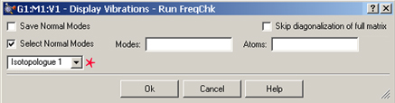
Figure 95. Running FreqChk to Perform Vibrational Analysis
This dialog is used to run the freqchk utility included with Gaussian. This utility performs vibrational analysis for the isotopologue specified in the popup menu in the left portion of the dialog (the menu is marked with a star); here the analysis will be performed for the second isotopologue. Once complete, the modes and spectra are available for visualization via the Display Vibrations dialog.
The Save Normal Modes and Select Normal Modes items are relevant only with Gaussian 09. They correspond to the Freq=SaveNormalModes and Freq=SelectNormalModes options, respectively (and to the equivalent FreqChk options). The former saves computed normal modes back to the checkpoint file, and the latter limits the vibrational analysis to the listed modes (Modes) and modes involving the listed atoms/atom types (Atoms). The Skip diagonalization of full matrix corresponds to Freq=NoDiagFull.
Once you exit the Run FreqChk dialog, the utility will run, and the Display Vibrations window will open. It is illustrated in Figure 96 as it appears after FreqChk completes.
The items in the top row of the dialog allow you to select which isotopologue’s data is displayed (the Active Data popup menu). The button opens the Run FreqChk dialog, and the button opens the Atom List Editor. See Figure 99 for an example of displaying vibrational data for multiple isotopologues.
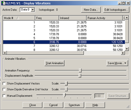
Figure 96. The Display Vibrations Window
This dialog displays a table of all computed spectra from frequency calculations. In this case, we see the vibrational frequencies, infrared intensities, Raman intensities and VCD rotational strengths. The window’s Spectrum button is used to access graphical representations of the predicted spectra.
The Display Vibrations dialog shows which vibration is currently selected for dynamic display. You can start this display by selecting the button, and halt it by clicking on the button. The molecule will begin a cyclical displacement showing the motions corresponding to the vibration selected. The two slide bars below the button adjust the speed and magnitude of the motion. Default values for these settings may be specified in the Vibrations Preferences panel (as well as for the displacement and dipole derivative unit vector which are discussed below).
The animation can also be saved as a movie and/or as individual frames using the button (see the discussion of saving movies earlier in this manual for more information).
You can select other modes by selecting the desired mode in the scrolling list. You can select a new mode without halting the previous one. You can also rotate and move the vibrating molecule, using the normal mouse buttons.
The Spectrum button presents Gaussian’s estimate of the spectrum in line format. Note that the intensity values are relative to the highest value in the present set, and bear no precise relationship to experimental band intensities. Example spectra are illustrated in Figure 97. Clicking on the various peaks within the spectra is another method for selecting which vibration mode is currently animated.
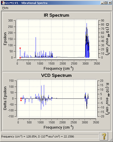
Figure 97. GaussView Spectra Displays
These plots display the IR and VCD spectra graphically. The available spectra depend on the Gaussian calculation that was run.
Vector-Based Displays
The two vector-related checkboxes in the bottom section of the Display Vibrations dialog have the following meanings (see Figure 87 for examples):
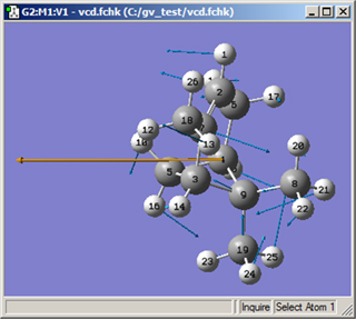
Figure 98. Displaying the Displacement Vector and Dipole Derivative Unit Vector
The various displacement vectors are displayed in blue, and the dipole derivative unit vector is the orange arrow on the left.
Using Manual Displacement Display Mode
The Manual Displacement box allows you to set the displacement as desired. When it is checked, animation of the vibration will be turned off. When checked, the slider, number box, and button become active. In this mode, changing the slider or the corresponding number box will cause the molecule to be statically displaced along the currently active normal mode. The center value of the slider, or zero in the text box, corresponds to no displacement. Moving the slider to the right or entering a positive value in the text box will displace the atoms along the currently active normal mode. Moving to the left or entering a negative value will displace the atoms in the direction opposite of the currently active normal mode. The range of values allowed in the text box ranges from -1 to +1. Clicking on will cause a new molecule window to appear with a geometry exactly corresponding to the displaced structure.
The primary use of this tool is to help eliminate spurious negative eigenvalues. hen one is searching for a transition state, it is not uncommon to end up with a structure containing two (or more) negative eigenvalues instead. These spurious negative eigenvalues are generally small but must be eliminated to isolate the true transition state. For these cases, select the normal mode corresponding to the spurious negative eigenvalue, and then select Manual Displacement. Adjust the slider to the right (or enter a positive number in the text box), and then select to create a new molecule with the displaced geometry, which you can then reoptimize. If a positive displacement fails to eliminate the spurious negative eigenvalue, follow the same procedure with a displacement in the negative direction. You can also try varying the magnitude of the displacement.
A second purpose of manual displacement is to generate pictures of a molecule in the midst of a vibration. Thus, it can be used to effectively freeze the animation of the vibration at a specific point.
Comparing Spectra for Isotopologues
GaussView makes it easy to compare spectra for different isotopologues of the same structure. To do so, you first define the desired isotopes for each isotopologue using the Atom List Editor. Then you generate vibrational data sets for each one. Once completed, you can use the Display Vibrations dialog to examine the spectra and normal modes.
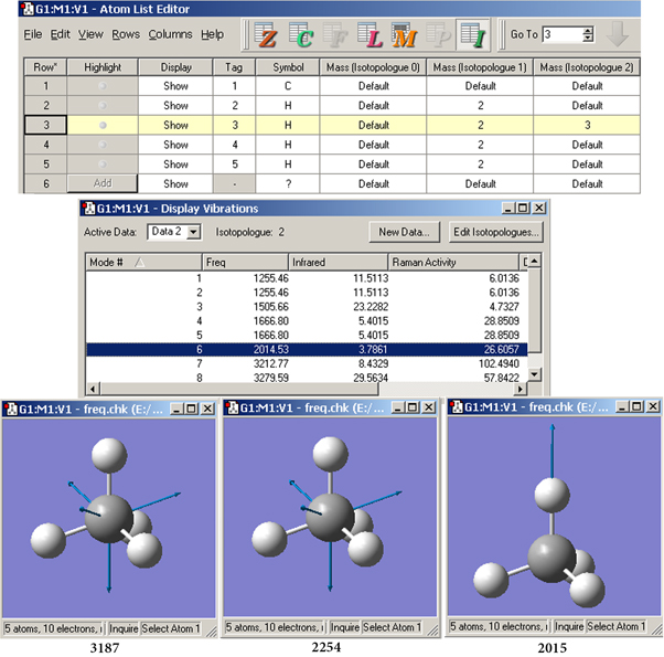
Figure 99. Setting Up Isotopologues and Comparing Normal Modes
In the Atom List Editor (top), we have defined three isotopologues for this simple molecule: one with the standard isotopes, one with deuterium replacing each hydrogen, and a third with tritium replacing a single hydrogen. The normal mode corresponding to the sixth frequency shifts location for each isotopologue (compare the values beneath each View window). The motion for the first two isotopologues is similar, but the mode for the tritium form has the motion confined to that atom.
Frequency-Dependent Calculation Results
Gaussian frequency calculations can specify values for the electromagnetic field perturbation at which to compute vibration properties. GaussView allows you to specify the desired incident light frequency for such frequency-dependent calculations by adding a popup menu to the top of the Display Vibrations window, as illustrated in Figure 100.
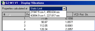
Figure 100. Specifying a Specific Frequency
GaussView adds this menu at the top of the Display Vibrations window for frequency-dependent calculation results. The Static Limit selection corresponds to a standard frequency calculation.
The Results=>NMR menu item displays the spectrum from an NMR calculation. An example spectrum is shown in Figure 101.
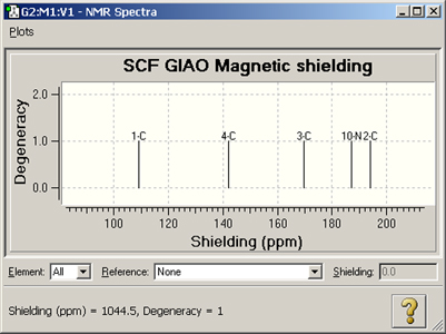
Figure 101. NMR Spectrum Display
This is the default NMR display format. It displays all computed peaks. Clicking on a peak with the cursor displays the shielding value and degeneracy in the lower left corner of the window (e.g., peak 2-C above)
The fields at the bottom of the NMR Spectra window allow you to view the same data as relative values with respect to TMS or other standards (see Figure 102). To use this feature, first select the desired element in the leftmost popup menu, and then select one of the available standard calculation results from the Reference field. The peaks will then reflect relative values with respect to the selected reference.
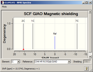
Figure 102. Displaying NMR Chemical Shifts
Clicking on a peak in this display mode shows the numeric chemical shift with respect to the specified standard in the lower left corner of the window. The corresponding shielding value is displayed in the Shielding field.
The Results=>UV-VIS menu item displays the spectra computed by an excited states calculation. An example spectrum is displayed in Figure 103.
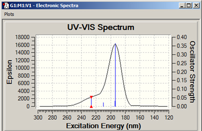
Figure 103. Example UV-Visible Spectrum Display
Additional spectra may be viewed for excited states calculations, including ECD for chiral molecules.
Viewing Optimization Results and Other Structure Sequences
When you open a results file containing such results from optimizations, potential energy surface scans, IRC calculations or ADMP or BOMD trajectory calculations, you will need to check the Read intermediate geometries (optimization only) checkbox in the Open File dialog in order to retrieve all of the geometries that are present (see Figure 104). When you do so, each geometry that is present becomes a separate model within a new molecule group (by default). Note that this checkbox applies to all of these job types, despite being labeled optimization only.
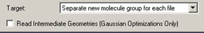
Figure 104. Retrieving Intermediate Results from Optimizations and Similar Jobs
The setting in the Target field above is the recommended one for opening files containing multiple structures. Don’t forget to check the Read intermediate geometries checkbox, or only the final structure will be retrieved.
You can animate the various structures using the buttons in the View window’s toolbar when the View window is set to single model mode. Animation begins by pressing the green circle button in the toolbar. The animation can then be stopped via the red X icon which replaces it. The animation speed is controlled by the Animation Delay setting in the General panel of the Display preferences.
The remaining items on the Results menu (Scan, IRC, Trajectory, Optimization) all allow you to view plots of energy and other results from calculations that produce multiple structures among their results. Figure 105 illustrates the displays for a geometry optimization.
The specific plots that appear vary by job type:
You can click on the various points in the plot, and the corresponding structure will appear in the View window.
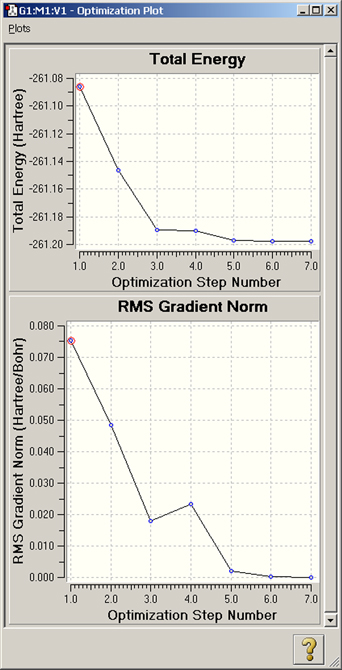
Figure 105. Plots from a Geometry Optimization
These plots display the total energy and root-mean-square gradient for each optimization point
Viewing 3D Plots of 2-Variable Scan Calculations
Gaussian Scan calculations over two variables are plotted by GaussView as three dimensional surfaces. An example appears in Figure 106. You can click on the various points in this plot as for 2D plots.
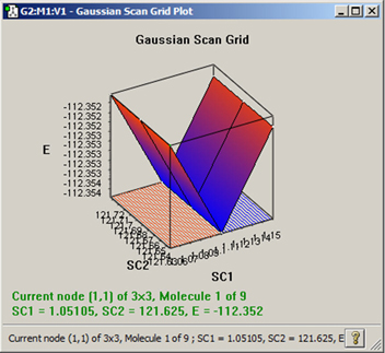
Figure 106. Results Plot for a PES Scan over 2 Variables
Only scan calculations over exactly two variables will produce plots like this one. Note that this plot can be rotated and zoomed using the standard mouse actions.
Plotting Additional Properties
You can create additional plots of various properties for these job types. This is done by selecting the Plots=>Plot Molecular Property menu item in the plot window. This results in the dialog in Figure 107.
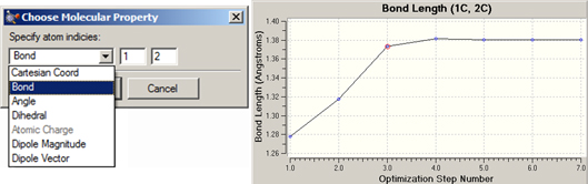
Figure 107. Creating An Additional Plot
In this example, we are adding a plot displaying the C-C bond distance for atoms 1 and 2 over the course of the geometry optimization. The dialog at the left displays the various items that may be plotted.
The items available for plotting vary by the job type. Once generated, the new plot appears below the standard ones in the plots window.
Correcting Plot Discontinuities
When data is read in for a multi-geometry plot, the values along the X-axis should form a single continuous ascending set. In some occasions, a user may include molecules from two or more different files within the same molecule group. This is sometimes useful for comparison purposes or to extend the output from a previous run. When this occurs, the X-axis values will no longer form a single continuous ascending set, resulting in a jagged appearance in the resulting plot. When this situation is detected, an informational message is displayed.
The Plots=>Fix Discontinuity menu item may be used to correct such plots. When this feature is used, the words “(Modified)” are added to the title of the plot to remind the user that the data in the plot has been modified and so should be viewed with caution.
Manipulating and Customizing Plots and Spectra
All plots and spectra can be manipulated for viewing in a variety of ways:
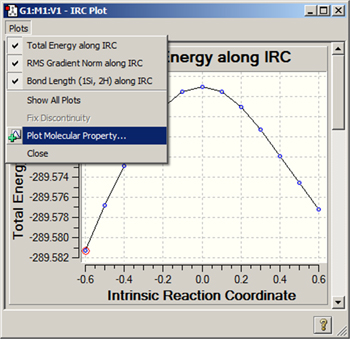
Figure 108. The Plots Menu
This menu is found in all plot and spectra windows. This particular example comes from the plots window displayed for an IRC calculation. Currently, all available plots are visible.
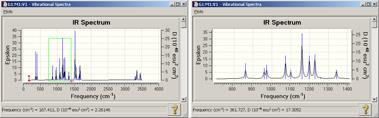
Figure 109. Zooming In on a Spectrum
The spectrum on the left is the one initially displayed by GaussView. Here, we are zooming in on the area in green. The resulting view is displayed on the right.
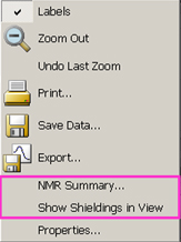
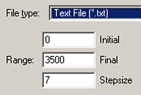
Figure 110. The Plot/Spectrum Context Menu and Save Data Range Fields
The menu on the left appears when you right click within a plot or spectrum. Only applicable items will be included and active. The fields on the right are added to the standard Save dialog when you select Save Data for a spectrum.
Customizing Plots and Spectra
Figure 111 appears when you select the Properties item from the context menu for a plot or spectrum.
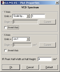
Figure 111. Customizing a Plot/Spectrum
This dialog may be used to customize many aspects of a plot or spectrum. Not all controls are active for all item types. Note that the field at the bottom of the dialog varies according to the spectrum type (here, we are working on a vibrational spectrum).
The various controls in the dialog have the following effects:
Other fields that may appear in the dialog include the following:
The context menu for plots and spectra contains the Save Data item. This may be used to save the numeric data corresponding to a plot/spectrum to an external file. Here is an example of the data saved from an IR spectrum:
# IR Spectrum
# X-Axis: Frequency (cm-1)
# Y-Axis: Epsilon
#           X               Y               DY/DX
    1400.0000000000    0.2434072675      0.0040413306
    1404.0000000000    0.2604146278      0.0044720368
    1408.0000000000    0.2792680154      0.0049661578
    …
You can specify the range of data and step size between points for this kind of data via the additional fields that GaussView adds to the standard Save dialog (illustrated to the right of the data above).
Data from plots of geometry optimizations, IRC calculations and the like can be saved in the same way. Here is some example data from an IRC calculation:
# Total Energy along IRC
# X-Axis: Intrinsic Reaction Coordinate
# Y-Axis: Total Energy (Hartree)
#         X                   Y
   -0.5999778220      -289.5812430000
   -0.4999857200      -289.5768190000
   -0.3999923250      -289.5728940000
   ...
For NMR spectra, an additional summary file may also be written, using the NMR Summary item on the spectrum’s context menu. Here is an example:
# Summary of NMR spectra ( SCF GIAO Magnetic shielding)
# Degenerate peaks are condensed together (Degeneracy Tolerance 0.05)
#
#          Shielding (ppm)     Degeneracy    Elem    Atoms
            26.6182000000        1.0000       H        1
            27.7949000000        2.0000       H       5,6
            76.9883000000        1.0000       C        2
            93.9401000000        1.0000       C        3
           106.1777000000        1.0000       C        4